Introduction
Before you can start working away on legal data science problems, you need to become familiar with the programming language that we will use in this course – R.
Why R?
Learning a programming language is an investment. So you may ask yourself: is it really worth it? And why R and not another language?
First, learning a programming language gives you a sense of what programmers do. Most people interact with technology through beautiful user-interfaces. Yet, all this technology was built with programming code. Then, just as you do not learn how to cook by eating, you need to try coding yourself to get a sense of what it takes to run computations or to build a beautiful interface.
Second, R was chosen for this course because it enables you to work on the entire life cycle of a legal data science project in one environment – from scraping a website to conducting your analysis to producing appealing visualizations and online applications. Other coding-for-lawyers courses use Python, which is also a good choice. Keep in mind that while programming languages differ, they are based on very similar principles. So if you know how to code in R, you will find it much easier to learn Python, for example.
Finally, another reason to choose R is because of it is an open source product with an active user community. Researchers and programmers create new functionalities for R (so called “R packages”) every day. We will use such R packages in many of our lessons. Moreover, because of its active user community there are many resources available online that will help you solve any problems that you may encounter.
What we do in this lesson
We get you started. In this first lesson, you will learn about basic concepts and operations in R:
1. Basic Calculations in R
2. Data types and functions
3. Accessing and manipulating data
4. Plotting data
5. Basic string operations
6. Loops
If you have not worked with R before, please take the time to complete this lesson and its exercises. It will make it easier to follow the subsequent lessons.
Useful Resources
A great book to get you started with R and its use in the humanities is:
Arnold, Taylor, and Lauren Tilton. Humanities Data in R: Exploring Networks, Geospatial Data, Images, and Text. 1st ed. 2015 edition. Cham: Springer, 2015.
R Script
Getting started
Version March 2018
This script provides a concise introduction to the basic functionalities of R.
R (and for that matter any programming language) is hard to grasp at first. The learning curve is steep, but it does get easier. Moreover, there are a multitude of free resources available online that provide guidance and support to learn on your own. Also disclaimer: I am law professor, not a programmer. So other resources will be better at teaching you how to program. However, if you are interested in learning how lawyers can use data science, and more specifically the R programming language, then keep on reading.Setting up R and RStudio
To get started, you will need to download two applications. First, you will need to download the program R here. Second, you should also download the user-friendly interface for working with R called RStudio here. A word on programming before we start. Programming is a bit like cooking using a recipe. The script is the recipe that you follow and the console is the stove you cook on. In other words, it is where you execute the code from your script. Like cooking your favorite recipe, the script will ensure that you can execute the same code today, in a week or in a year. You don't have to remember how you did it last time, instead, you just need to follow the steps in your script. Two consequences flow from this. First, whenever you make changes or try out new alternatives, write them in the script (or create a new script) and not in the console. Otherwise you risk losing the information how you did it. Second, make sure to make comments about your code to ensure that months from now you will be able to easily understand your work. This will make it easier to change your code or customize it to work with new data. In R, you comment with the "#" symbol as you will see below. Now, we are ready to go.Basic calculations in R
In simple terms, R is a calculator: You enter an equation and it returns the answer. Let's try this with a few examples. Type in "1+1" in your R console. Note that the ## below is the answer returned by R.1+1
## [1] 2
16/4
## [1] 4
6^8.5
## [1] 4114202
# This is my first calculation in R:
1+1
## [1] 2
x <- 1
y <- 2+2
y
## [1] 4
print(y)
## [1] 4
x+y
## [1] 5
silly_name <- 5+3
silly_name
## [1] 8
Object classes
R powerful is a powerful tool because you can work with numbers and with other types of data. More specifically there are three types of data objects that we will use.- - numerical objects e.g. 1; 67; 5.56541
- - logical objects i.e. TRUE, FALSE
- - character objects e.g. "Hello World"
# To determine the type of data object you simply ask class().
                            class
                            (silly_name)
## [1] "numeric"
                            another_silly_name
                            <-
                            "Hello World"
class
                            (another_silly_name)
## [1] "character"
# Whenever you do not know what a function does you can ask using "?".
?class()
# To do so you aggregate values with c().
numeric_vector <- c ( 1 , 2 , 3 , 4 , 5 )
numeric_vector
## [1] 1 2 3 4 5
# A more efficient way to create the same vector would be:
numeric_vector <- c ( 1 : 5 )
numeric_vector
## [1] 1 2 3 4 5
# You can create vectors with character strings, too.
character_vector <- c ( "Days" , "Months" , "Year" )
character_vector
## [1] "Days" "Months" "Year"
# As an example, take a look at one of the in-built dataframe of R ("USArrests") that provides crime statistics of US states.
data("USArrests")
print(USArrests)
##
| State | Murder | Assault | Urban Population | Rape |
|---|---|---|---|---|
| Alabama | 13.2 | 236 | 58 | 21.2 |
| Alaska | 10.0 | 263 | 48 | 44.5 |
| Arizona | 8.1 | 294 | 80 | 31.0 |
| Arkansas | 8.8 | 190 | 50 | 19.5 |
| California | 9.0 | 276 | 91 | 40.6 |
| Colorado | 7.9 | 204 | 78 | 38.7 |
| Connecticut | 3.3 | 110 | 77 | 11.1 |
| Delaware | 5.9 | 238 | 72 | 15.8 |
| Florida | 15.4 | 335 | 80 | 31.9 |
| Georgia | 17.4 | 211 | 60 | 25.8 |
| Hawaii | 5.3 | 46 | 83 | 20.2 |
| Idaho | 2.6 | 120 | 54 | 14.2 |
| Illinois | 10.4 | 249 | 83 | 24.0 |
| Indiana | 7.2 | 113 | 65 | 21.0 |
| Iowa | 2.2 | 56 | 57 | 11.3 |
| Kansas | 6.0 | 115 | 66 | 18.0 |
| Kentucky | 9.7 | 109 | 52 | 16.3 |
| Louisiana | 15.4 | 249 | 66 | 22.2 |
| Maine | 2.1 | 83 | 51 | 7.8 |
| Maryland | 11.3 | 300 | 67 | 27.8 |
| Massechusetts | 4.4 | 149 | 85 | 16.3 |
| Michigan | 12.1 | 255 | 74 | 35.1 |
| Minnesota | 2.7 | 72 | 66 | 14.9 |
| Mississippi | 16.1 | 259 | 44 | 17.1 |
| Missouri | 9.0 | 178 | 70 | 28.2 |
| Montana | 6.0 | 109 | 53 | 16.4 |
| Nebraska | 4.3 | 102 | 62 | 16.5 |
| Nevada | 12.2 | 252 | 81 | 46.0 |
| New Hampshire | 2.1 | 57 | 56 | 9.5 |
| New Jersey | 7.4 | 159 | 89 | 18.8 |
| New Mexico | 11.4 | 285 | 70 | 32.1 |
| New York | 11.1 | 254 | 86 | 26.1 |
| North Carolina | 13.0 | 337 | 45 | 16.1 |
| North Dakota | 0.8 | 45 | 44 | 7.3 |
| Ohio | 7.3 | 120 | 75 | 21.4 |
| Oklahoma | 6.6 | 151 | 68 | 20.0 |
| Oregan | 4.9 | 159 | 67 | 29.3 |
| Pennsylvania | 6.3 | 106 | 72 | 14.9 |
| Rhode Island | 3.4 | 174 | 87 | 8.3 |
| South Carolina | 14.4 | 279 | 48 | 22.5 |
| South Dakota | 3.8 | 86 | 45 | 12.8 |
| Tennessee | 13.2 | 188 | 59 | 26.9 |
| Texas | 12.7 | 201 | 80 | 25.5 |
| Utah | 3.2 | 120 | 80 | 22.9 |
| Vermont | 2.2 | 48 | 32 | 11.2 |
| Virginia | 8.5 | 156 | 63 | 20.7 |
| Washington | 4.0 | 145 | 73 | 26.2 |
| West Virginia | 5.7 | 81 | 39 | 9.3 |
| Wisconsin | 2.6 | 53 | 66 | 10.8 |
| Wyoming | 6.8 | 161 | 60 | 15.6 |
Accessing and Manipulating Data
There are different commands you can use to access data in your R objects, and their use differs slightly between object classes. # To access an item in a list, just indicate its place within the vector through [ ].
character_vector <- c("Days", "Months", "Year")
character_vector[2]
## [1] "Months"
# If you are unsure about the location of given information in a list, use the which() function.
which(character_vector == "Months")
##[1] 2
# So when you want to access data on "Arkansas" (4th row) on "Murder" (1st column), you would write:
USArrests[4,1]
## [1] 8.8
# If you are interested in all columns for Arkansas just leave the space behind the comma blank.
USArrests[4,]
##
| State | Murder | Assault | Urban Population | Rape |
|---|---|---|---|---|
| Arkansas | 8.8 | 190 | 50 | 19.5 |
# Similarly, if you are interested in murder rates for all states just leave the space in front of the comma blank.
USArrests[,1]
## [1] 13.2 10.0 8.1 8.8 9.0 7.9 3.3 5.9 15.4 17.4 5.3 2.6 10.4 7.2 2.2 6.0 9.7 15.4 2.1 11.3 4.4 12.1 2.7 16.1 9.0 6.0
# To access only the murder rates in the USArrests dataframe, you can call the column name:
USArrests["Murder"]
##
| State | Murder |
|---|---|
| Alabama | 13.2 |
| Alaska | 10.0 |
| Arizona | 8.1 |
| Arkansas | 8.8 |
| California | 9.0 |
| Colorado | 7.9 |
| Connecticut | 3.3 |
| Delaware | 5.9 |
| Florida | 15.4 |
| Georgia | 17.4 |
| Hawaii | 5.3 |
| Idaho | 2.6 |
| Illinois | 10.4 |
| Indiana | 7.2 |
| Iowa | 2.2 |
| Kansas | 6.0 |
| Kentucky | 9.7 |
| Louisiana | 15.4 |
| Maine | 2.1 |
| Maryland | 11.3 |
| Massachusetts | 4.4 |
| Michigan | 12.1 |
| Minnesota | 2.7 |
| Mississippi | 16.1 |
| Missouri | 9.0 |
| Montana | 6.0 |
| Nebraska | 4.3 |
| Nevada | 12.2 |
| New Hampshire | 2.1 |
| New Jersey | 7.4 |
| New Mexico | 11.4 |
| New York | 11.1 |
| North Carolina | 13.0 |
| North Dakota | 0.8 |
| Ohio | 7.3 |
| Oklahoma | 6.6 |
| Oregan | 4.9 |
| Pennsylvania | 6.3 |
| Rhode Island | 3.4 |
| South Carolina | 14.4 |
| South Dakota | 3.8 |
| Tennessee | 13.2 |
| Texas | 12.7 |
| Utah | 3.2 |
| Vermont | 2.2 |
| Virginia | 8.5 |
| Washington | 4.0 |
| West Virginia | 5.7 |
| Wisconsin | 2.6 |
| Wyoming | 6.8 |
# Alternatively, to access the data in a column in a dataframe we can also use the $ character:
USArrests$Murder
## [1] 13.2 10.0 8.1 8.8 9.0 7.9 3.3 5.9 15.4 17.4 5.3 2.6 10.4 7.2 2.2 6.0 9.7 15.4 2.1 11.3 4.4 12.1 2.7 16.1 9.0 6.0
# For instance, to again get the murder rates in Arkansas, you can write:
USArrests$Murder[4]
## [1] 8.8
# For instance, we want to create a new dataframe that only has the murder rate data.
murder_rate <- USArrests["Murder"]
# Or we want to exclude murder rates from our dataset. Then we can simply write [,-1] which will eliminate the first column.
other_crimes <- USArrests[,-1]
print(other_crimes)
##
| State | Assault | Urban Population | Rape |
|---|---|---|---|
| Alabama | 236 | 58 | 21.2 |
| Alaska | 263 | 48 | 44.5 |
| Arizona | 294 | 80 | 31.0 |
| Arkansas | 190 | 50 | 19.5 |
| California | 276 | 91 | 40.6 |
| Colorado | 204 | 78 | 38.7 |
| Connecticut | 110 | 77 | 11.1 |
| Delaware | 238 | 72 | 15.8 |
| Florida | 335 | 80 | 31.9 |
| Georgia | 211 | 60 | 25.8 |
| Hawaii | 46 | 83 | 20.2 |
| Idaho | 120 | 54 | 14.2 |
| Illinois | 249 | 83 | 24.0 |
| Indiana | 113 | 65 | 21.0 |
| Iowa | 56 | 57 | 11.3 |
| Kansas | 115 | 66 | 18.0 |
| Kentucky | 109 | 52 | 16.3 |
| Louisiana | 249 | 66 | 22.2 |
| Maine | 83 | 51 | 7.8 |
| Maryland | 300 | 67 | 27.8 |
| Massachusetts | 149 | 85 | 16.3 |
| Michigan | 255 | 74 | 35.1 |
| Minnesota | 72 | 66 | 14.9 |
| Mississippi | 259 | 44 | 17.1 |
| Missouri | 178 | 70 | 28.2 |
| Montana | 109 | 53 | 16.4 |
| Nebraska | 102 | 62 | 16.5 |
| Nevada | 252 | 81 | 46.0 |
| New Hampshire | 57 | 56 | 9.5 |
| New Jersey | 159 | 89 | 18.8 |
| New Mexico | 285 | 70 | 32.1 |
| New York | 254 | 86 | 26.1 |
| North Carolina | 337 | 45 | 16.1 |
| North Dakota | 45 | 44 | 7.3 |
| Ohio | 120 | 75 | 21.4 |
| Oklahoma | 151 | 68 | 20.0 |
| Oregan | 159 | 67 | 29.3 |
| Pennsylvania | 106 | 72 | 14.9 |
| Rhode Island | 174 | 87 | 8.3 |
| South Carolina | 279 | 48 | 22.5 |
| South Dakota | 86 | 45 | 12.8 |
| Tennessee | 188 | 59 | 26.9 |
| Texas | 201 | 80 | 25.5 |
| Utah | 120 | 80 | 22.9 |
| Vermont | 48 | 32 | 11.2 |
| Virginia | 156 | 63 | 20.7 |
| Washington | 145 | 73 | 26.2 |
| West Virginia | 81 | 39 | 9.3 |
| Wisconsin | 53 | 66 | 10.8 |
| Wyoming | 161 | 60 | 15.6 |
# So if we want to merge the two datasets again, we can do:
full_dataset <- cbind(murder_rate,other_crimes)
print(full_dataset)
##
| State | Murder | Assault | Urban Population | Rape |
|---|---|---|---|---|
| Alabama | 13.2 | 236 | 58 | 21.2 |
| Alaska | 10.0 | 263 | 48 | 44.5 |
| Arizona | 8.1 | 294 | 80 | 31.0 |
| Arkansas | 8.8 | 190 | 50 | 19.5 |
| California | 9.0 | 276 | 91 | 40.6 |
| Colorado | 7.9 | 204 | 78 | 38.7 |
| Connecticut | 3.3 | 110 | 77 | 11.1 |
| Delaware | 5.9 | 238 | 72 | 15.8 |
| Florida | 15.4 | 335 | 80 | 31.9 |
| Georgia | 17.4 | 211 | 60 | 25.8 |
| Hawaii | 5.3 | 46 | 83 | 20.2 |
| Idaho | 2.6 | 120 | 54 | 14.2 |
| Illinois | 10.4 | 249 | 83 | 24.0 |
| Indiana | 7.2 | 113 | 65 | 21.0 |
| Iowa | 2.2 | 56 | 57 | 11.3 |
| Kansas | 6.0 | 115 | 66 | 18.0 |
| Kentucky | 9.7 | 109 | 52 | 16.3 |
| Louisiana | 15.4 | 249 | 66 | 22.2 |
| Maine | 2.1 | 83 | 51 | 7.8 |
| Maryland | 11.3 | 300 | 67 | 27.8 |
| Massachusetts | 4.4 | 149 | 85 | 16.3 |
| Michigan | 12.1 | 255 | 74 | 35.1 |
| Minnesota | 2.7 | 72 | 66 | 14.9 |
| Mississippi | 16.1 | 259 | 44 | 17.1 |
| Missouri | 9.0 | 178 | 70 | 28.2 |
| Montana | 6.0 | 109 | 53 | 16.4 |
| Nebraska | 4.3 | 102 | 62 | 16.5 |
| Nevada | 12.2 | 252 | 81 | 46.0 |
| New Hampshire | 2.1 | 57 | 56 | 9.5 |
| New Jersey | 7.4 | 159 | 89 | 18.8 |
| New Mexico | 11.4 | 285 | 70 | 32.1 |
| New York | 11.1 | 254 | 86 | 26.1 |
| North Carolina | 13.0 | 337 | 45 | 16.1 |
| North Dakota | 0.8 | 45 | 44 | 7.3 |
| Ohio | 7.3 | 120 | 75 | 21.4 |
| Oklahoma | 6.6 | 151 | 68 | 20.0 |
| Oregan | 4.9 | 159 | 67 | 29.3 |
| Pennsylvania | 6.3 | 106 | 72 | 14.9 |
| Rhode Island | 3.4 | 174 | 87 | 8.3 |
| South Carolina | 14.4 | 279 | 48 | 22.5 |
| South Dakota | 3.8 | 86 | 45 | 12.8 |
| Tennessee | 13.2 | 188 | 59 | 26.9 |
| Texas | 12.7 | 201 | 80 | 25.5 |
| Utah | 3.2 | 120 | 80 | 22.9 |
| Vermont | 2.2 | 48 | 32 | 11.2 |
| Virginia | 8.5 | 156 | 63 | 20.7 |
| Washington | 4.0 | 145 | 73 | 26.2 |
| West Virginia | 5.7 | 81 | 39 | 9.3 |
| Wisconsin | 2.6 | 53 | 66 | 10.8 |
| Wyoming | 6.8 | 161 | 60 | 15.6 |
Plotting Data
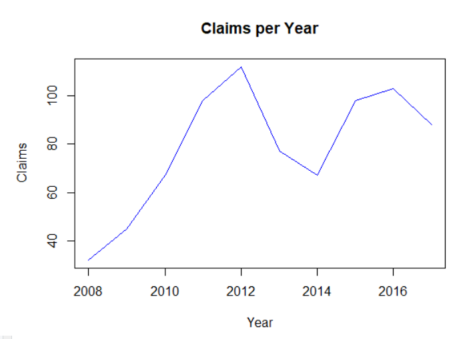
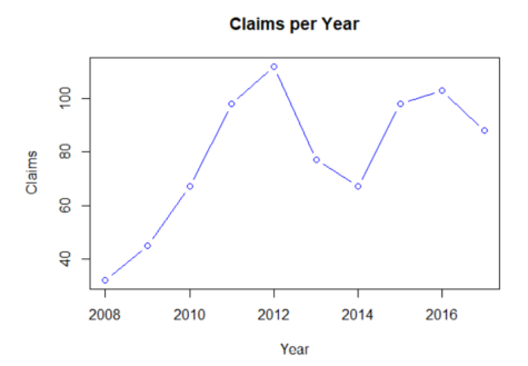
R is also great for data visualization. Here are a few simple graphs.# Let's create the following dataset of numbers of claims per year:
year <- c(2008:2017)
claims <- c(32,45,67,98,112,77,67,98,103,88)
disputes <- data.frame(year, claims)
print(disputes)
##
| Year | Claim | |
|---|---|---|
| 1 | 2008 | 32 |
| 2 | 2009 | 45 |
| 3 | 2010 | 67 |
| 4 | 2011 | 98 |
| 5 | 2012 | 112 |
| 6 | 2013 | 77 |
| 7 | 2014 | 67 |
| 8 | 2015 | 98 |
| 9 | 2016 | 103 |
| 10 | 2017 | 88 |
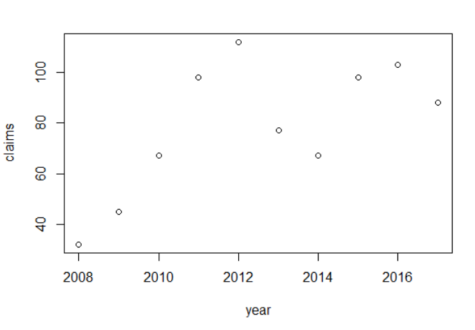
# We can visualize that data using the plot() function.
plot(disputes)
##
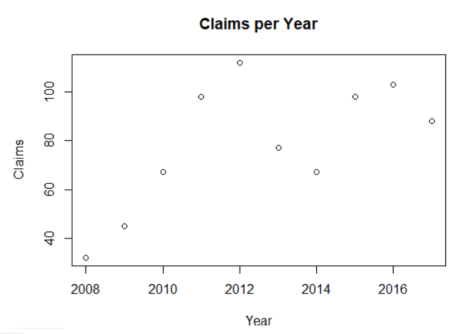
# Consult the R documentation to learn how the function can be further customized.
?plot()
plot(disputes$year,disputes$claims, type = "p", xlab="Year", ylab="Claims",
     main = "Claims per Year")
##
plot(disputes$year,disputes$claims, type = "b", col="blue", xlab="Year", ylab="Claims",
     main = "Claims per Year")
##
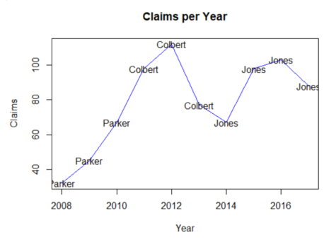
judges <- c("Parker","Parker","Parker","Colbert","Colbert","Colbert","Jones","Jones","Jones","Jones")
# Let's add the judge data to our dataframe and print the data again.
disputes <- cbind(disputes, judges)
print(disputes)
##
| Year | Claim | Judges | |
|---|---|---|---|
| 1 | 2008 | 32 | Parker |
| 2 | 2009 | 45 | Parker |
| 3 | 2010 | 67 | Parker |
| 4 | 2011 | 98 | Colbert |
| 5 | 2012 | 112 | Colbert |
| 6 | 2013 | 77 | Colbert |
| 7 | 2014 | 67 | Jones |
| 8 | 2015 | 98 | Jones |
| 9 | 2016 | 103 | Jones |
| 10 | 2017 | 88 | Jones |
# We can add the name of the judges to the plot with the text() function.
plot(disputes$year,disputes$claims, type = "l", col="blue", xlab="Year", ylab="Claims",
     main = "Claims per Year")
text(disputes$year,disputes$claims, label=disputes$judges)
Basic String Operations
In this course, we will often be dealing with text data. These are also called character strings in R.
example <- "Hello World"
To merge two strings we can use the paste() function. This function uses a separator which is by default " ".
new_example <- paste("Hello World", "how is your day")
##[1] "Hello World how is your day"
We can also change that separator.
new_example <- paste("Hello World", "how is your day", sep=", ")
new_example
##[1] "Hello World, how is your day"
To split a string we can use the strsplit() function.
strsplit(new_example, ",")
##[1] "Hello World" " how is your day"
When using the strsplit()function, R returns us a nested list. To access only the elements of the sublist we can ask for the first element in the sublist [[1]].
strsplit(new_example, ",")[[1]]
## [1] "Hello World" " how is your day"
As you will see in the remainder of the course, some functions return nested lists. This is a frequent source of trouble for people who are new to R. So if you have difficulties accessing specific elements in a vector, check to see whether you are dealing with a sublist.
Loops
It is often useful to apply a function to all of the elements in a vector or a data frame, rather than just applying it to one. For that we use a loop. Imagine you want to multiply the numbers 20 to 29 by 13. You can write 20*13, 21*13, 22*13 ... A loop does that work for you.
# Let's first create a list of numbers from 20 to 29.
number_list <- c(20:29)
print(number_list)
## [1] 20 21 22 23 24 25 26 27 28 29
for (element in number_list) {
print(element*13)
}
 ##
[1] 260
[1] 273
[1] 286
[1] 299
[1] 312
[1] 325
[1] 338
[1] 351
[1] 364
[1] 377
length(number_list)
## [1] 10
# So we can write: for the ranks from 1 to length of list (here 10), perform a function on each element of that rank.
for (rank in 1:length(number_list)) {print(number_list[rank]*13)}
 ##
[1] 260
[1] 273
[1] 286
[1] 299
[1] 312
[1] 325
[1] 338
[1] 351
[1] 364
[1] 377
# This yields the last value of the numbered list i.e. 29.
print(element)
## [1] 29
# This yields the last position of the numbered list i.e. 10.
print (rank)
##[1] 10
# This is just a sample dataframe with 3 rows and 4 columns:
sample_dataframe <- as.data.frame(matrix(data=1:12, nrow=3, ncol=4, byrow=FALSE))
print(sample_dataframe)
##
  V1 V2 V3 V4
1 1 4 7 10
2 2 5 8 11
3 3 6 9 12
# FOR the rows IN row number 1 to the total number of rows in my sample_dataframe
# PRINT the SUM of each row.
for (row in 1:nrow(sample_dataframe)) {
print(sum(sample_dataframe[row,]))
}
 ##
[1] 22
[1] 26
[1] 30
# To do the same thing for column sums, we just need to (1) adjust for the number of columnes (ncol) and (2) adjust the comma. Note that I also changed "row" to "col" but this is not necessary. But it helps understanding what is being done.
for (col in 1:ncol(sample_dataframe)) {print(sum(sample_dataframe[,col]))
}
## [1] 6 [1] 15 [1] 24 [1] 33
Dataset
There are no datasets for this lesson.
Exercises
There are a couple of sample dataframes in R. For this exercise, we will work with some of them. We will also train your “help yourself” instincts. There is ample help on the web. Platforms like stackoverflow provide great answers to most of your R-related questions.
Let’s give it a try.
Example 1)
                            # Load the data set on USA Arrest rates.
                            data
                            (
                            "USArrests"
                            )
Answer the following questions (with the help of online resources).
- Sort the data by the Murder rate. Which state has the highest murder rate?
- What is the average murder rate across all states?
- What is the correlation between urban population and murder rates?
Example 2)
                            # Let's look at some data on judges.
                            data
                            (
                            "USJudgeRatings"
                            )
- What judge has the highest overall rating?
- Which category is the highest rated overall?
Example 3)
                            # Finally, let's take a look at Canada and the Canadian lynx dataset.
                            data
                            (
                            "lynx"
                            )
- Plot the number of lynx hunted every year.
- Try different plot types. Which visualization is most appropriate?
